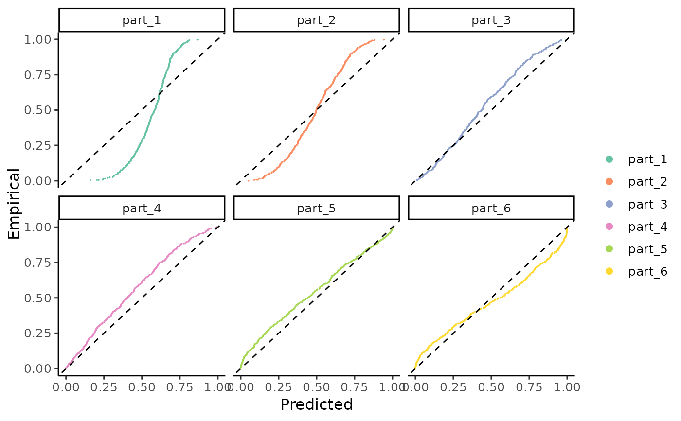
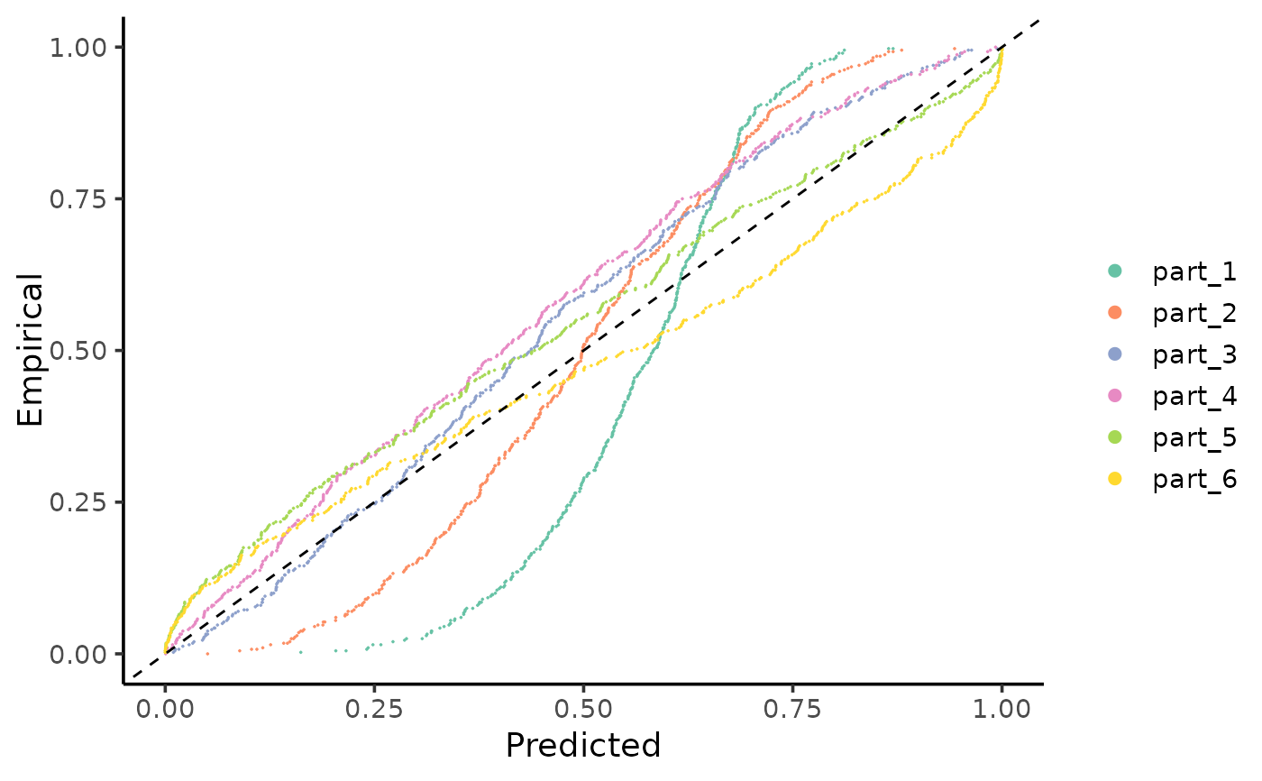
Plots the cumulative distributions of PIT-values for local calibration diagnostics.
Source:R/gg_CD_local.R
gg_CD_local.RdThis function generates a ggplot visual representation to compare the predicted versus empirical cumulative distributions of Probability Integral Transform (PIT) values at a local level. It is useful for diagnosing the calibration in different regions within the dataset, since miscalibration patterns may differ across the covariate space. The function allows for customization of the plot layers to suit specific needs. For advanced customization of the plot layers, refer to the ggplot2 User Guide.
Arguments
- pit_local
A data frame of local PIT-values, typically obtained from
PIT_local().- mse
Mean Squared Error calculated from the calibration dataset.
- psz
Double indicating the size of the points on the plot. Default is 0.001.
- abline
Color of the diagonal line. Default color is "red".
- pal
Palette name from RColorBrewer for coloring the plot. Default is "Set2".
- facet
Logical value indicating if a separate visualization for each subgroup is preferred. Default is FALSE.
- ...
Additional parameters to customize the ggplot.
Value
A ggplot object displaying the cumulative distributions of PIT-values that that can be customized as needed.
Details
This funcion will work with the output of the PIT_local() function, which provides the PIT-values for each subgroup pf the covariate space in the appropriate format.
Examples
n <- 10000
split <- 0.8

mu <- function(x1){
10 + 5*x1^2
}

sigma_v <- function(x1){
30*x1
}


x <- runif(n, 1, 10)
y <- rnorm(n, mu(x), sigma_v(x))

x_train <- x[1:(n*split)]
y_train <- y[1:(n*split)]

x_cal <- x[(n*split+1):n]
y_cal <- y[(n*split+1):n]

model <- lm(y_train ~ x_train)

y_hat <- predict(model, newdata=data.frame(x_train=x_cal))

MSE_cal <- mean((y_hat - y_cal)^2)

pit_local <- PIT_local(xcal = x_cal, ycal=y_cal, yhat=y_hat, mse=MSE_cal)

gg_CD_local(pit_local, mse=MSE_cal)

gg_CD_local(pit_local, facet=TRUE, mse=MSE_cal)