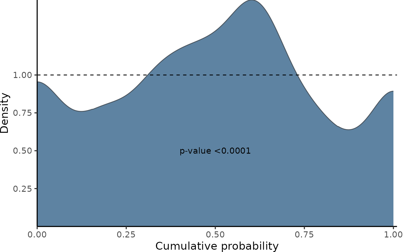
Plots Density Distributions of PIT-values for Global Calibration Diagnostics

This function generates a ggplot visual representation of the density of Probability Integral Transform (PIT) values globally. For advanced customization of the plot layers, refer to the ggplot2 User Guide.

Usage

gg_PIT_global(
  pit,
  type = "density",
  fill = "steelblue4",
  alpha = 0.8,
  print_p = TRUE
)

Arguments

pit: Vector of PIT values to be plotted.
type: Character string specifying the type of plot: either "density" or "histogram". This determines the representation style of the PIT values.
fill: Character string defining the fill color of the plot. Default is 'steelblue4'.
alpha: Numeric value for the opacity of the plot fill, with 0 being fully transparent and 1 being fully opaque. Default is 0.8.
print_p: Logical value indicating whether to print the p-value from the Kolmogorov-Smirnov test. Useful for statistical diagnostics.

Value

A ggplot object depicting a density graph of PIT-values, which can be further customized.

Details

This function also tests the PIT-values for uniformity using the Kolmogorov-Smirnov test (ks.test). The p-value from the test is printed on the plot if print_p is set to TRUE.

Examples


n <- 10000
split <- 0.8

# generating heterocedastic data
mu <- function(x1){
10 + 5*x1^2
}

sigma_v <- function(x1){
30*x1
}

x <- runif(n, 1, 10)
y <- rnorm(n, mu(x), sigma_v(x))

x_train <- x[1:(n*split)]
y_train <- y[1:(n*split)]

x_cal <- x[(n*split+1):n]
y_cal <- y[(n*split+1):n]

model <- lm(y_train ~ x_train)

y_hat <- predict(model, newdata=data.frame(x_train=x_cal))

MSE_cal <- mean((y_hat - y_cal)^2)

pit <- PIT_global(ycal=y_cal, yhat=y_hat, mse=MSE_cal)

gg_PIT_global(pit)